Spurious Solution Suppression: the Goldilocks upwind discontinuous Galerkin Time-domain method

There are roughly three schools of thought about how much stabilization should be added to control the continuity of solutions obtained through discontinuous Galerkin discretizations of time-dependent linear wave problems (e.g. acoustics, electromagnetics, linear elasticity).

We can view each of these methods as one instance of a singly parameterized method. Without dwelling on too many details the variational equation for a symmetric linear hyperbolic wave system on each element is

Here q is a state vector approximated by polynomials of degree N on element D^e. The parameter tau is a tunable non-negative quantity. In this blog entry we consider three values for tau that appear in the literature (albeit in slightly different presentations).

Approach #1 (tau=0): the central flux community favors "central flux" formulations which do not actively control continuity of the solution between the faces of neighboring elements. The neat side effect of this choice is that for symmetric hyperbolic wave systems a total energy will be conserved. This choice allows for the use of symplectic time integration schemes, for instance leap-frog schemes.

Approach #2 (tau=1): the upwind flux community favors a stabilizing term that penalizes any "un-physical" jumps in the solution. The stabilization is not instantaneous and takes time to relax away jumps in the solution. The eigenvalues of upwind discretizations are typically complex necessitating the use of a time-stepping method with region of absolute stability that extends into the left half of the complex plane.

Approach #3 (tau=infinity): the classical finite element community prefers solutions to be continuous at element interfaces. This can be emulated in DGTD simulations through an infinitely penalizing flux. This acts to instantaneously damp jumps that are not in the null spaces of the normal flux matrix D. This forces the solution into a continuous (or semi-continuous) subspace of the usual broken DG approximation space depending on the structure of D.

In the following plots we illustrate the sensitivity of the complex valued eigenvalues of a DGTD spatial wave transport operator to the penalty constant. In the first image we show that as the penalty increases from zero to a large value that

1. some eigenvalues shift to the left half plane corresponding to strongly damped eigenmodes of the operator that are related to saw tooth modes.

2. some eigenvalues stay on the imaginary axis corresponding to nearly continuous and physically realistic eigenmodes for the wave problem.

3. some eigenvalues start on the imaginary axis for the central DGTD method (but unfortunately correspond to spurious discrete eigenmodes) are damped with increasing penalty, until they turn around and head towards the imaginary axis and become spurious continuous eigenmodes.

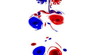
The following image shows that some eigenmodes are heavily damped

The next image zooms into the vicinity of the imaginary axis. It shows that as the tau parameter increases modes start as blue circles for tau=0, track through the triangle upwind eigenvalues at tau=1, and that some return to the imaginary axis for large tau.

The key observation is that the heavy black lines represent eigenvalue tracks as the tau parameter varies. The worrying tracks are those that start as high frequency imaginary values and work there way left into the left half of the complex plane and then carry on back towards the imaginary axis at a lower frequency to once again become persistent spurious but this time interlaced in the resolved spectrum.

In summary: if the penalty coefficient, tau, is too small then spurious oscillatory modes persist in time. If tau is too large then these modes are converted into continuous but still spurious oscillatory modes. However, with the small but non-zero "goldilocks" penalty that upwind fluxes employ these unphysical modes will be damped in time.

Reference: see this arXiv.org preprint of this journal article for a deeper dive into the mathematical details.